Intro to GIS: Final Project - GIS Analysis: Bobwhite-Manatee Transmission Line

     The skills I have learned throughout the semester culminated in this final project. As a class, we were asked to put ourselves in the shoes of a GIS Analyst seeking employment. Thus, we are to demonstrate our aptitude with the presentation of previous work.

     This project required organization of a large amount of data, working with acquired data, and generating new datasets. I also needed to ensure that I could communicate the results of my analyses effectively through a presentation involving appropriate visual aids (maps, charts, tables, etc). To aid in all that organization I used a file geodatabase. There are many advantages to using a file geodatabase. While I was the only person working in this geodatabase, in a professional setting I may have had to coordinate my efforts with others. The geodatabase makes it easier to accomplish group editing and works cross-platform.

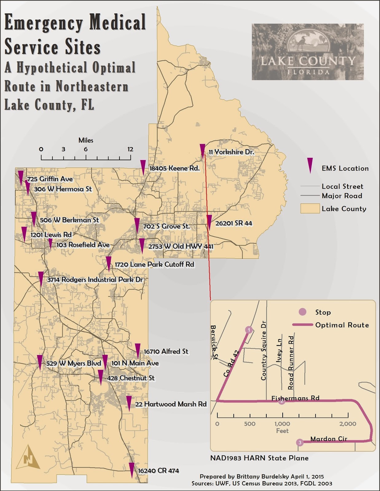
A map I created to examine the impact of a proposed
transmission line on existing conservation lands.

     The analysis portion of this project was carried out in ArcGIS and I used PowerPoint to assemble  a presentation for my prospective employer [here is a link to the transcript]. Additionally, I used Excel to summarize the resulting data and compose various visual aids such as pie charts and bar graphs.

     The goal of the analysis was to determine the impact and feasibility of a transmission line that spanned two counties, Manatee and Sarasota, in Florida. I set out to determine if the proposed corridor for the line avoided large areas of environmentally sensitive lands, if it had relatively few home in close proximity, generally avoided schools, and if it could be built at a reasonable cost. The analyses I carried out (a combination of location and attribute queries, overlay analyses, etc) showed that the transmission line met all of these objectives which results in an overall minimal impact on the surrounding community.

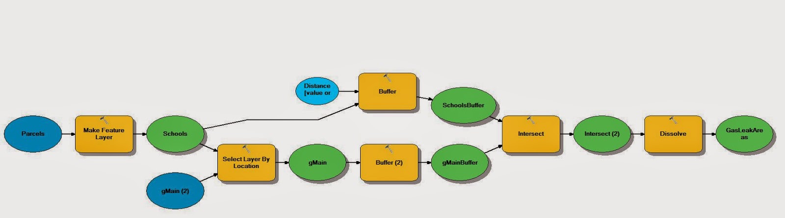
One of the maps I created for the analysis of the impact
of a transmission line on its surrounding community. 

Above, to the right, and below, I have placed examples of some of the maps and a pie chart that I used in my presentation. This project took many hours and gave me insight into what it will be like to do analytic work using GIS in the real world. I now have a serious appreciation for all of the effort and coordination that go into utilities projects. (I wonder how they did it before GIS). I hope that you enjoy my presentation and thank you for visiting my blog. It has been a great semester filled with all things GIS (and cartography).

One of the charts I created to help summarize the results of an analysis of the impact of a transmission line corridor on land owners/residents.

In case you missed the links above, here are additional ones:
Presentation
Transcript

   
Thanks again for keeping up with me.

Cartography: Final Project - Thematic Mapping of Two Sets of Data

 Map Content   

     This is the last project for this course. The culmination of this project is a single map displaying two datasets. As a final, it tests our ability to design and implement cartographic analyses independently while integrating skills learned throughout the semester. We were given the choice of two data sources (either SAT or ACT testing data), each with two sets of data to map. I chose to use the testing data published by ACT, Inc. I mapped average test score and percentages of graduates tested, by state.
     I used Excel to create a table that could be subsequently imported into ArcMap and joined to the basemap data. I analyzed the data in Excel to see if it was normally distributed. It turns out that neither dataset is normal. (This can be attributed to the fact that in some states taking this test was a requirement while in other states participation is voluntary. Participation in turn affects the average score since more students [of varying aptitudes] are taking the exams in the mandatory states the average score is representative of a broader student base). This is important when considering how to classify and portray your data. After this preliminary data analysis, I worked on preparing my basemap. The basemap data comes from the US Census Bureau and lack a projection. I used Albers Equal Area Conic as it is appropriate for this landmass and the preservation of area (important for preserving the enumeration unit in choropleth maps which is how I wanted to map part of the data).     

     Perhaps the data could have been better represented in a different way but I intuitively leaned toward a chorpoleth basemap and some sort of proportional or graduation symbology. I decided to map the percentage data on a choropleth map while representing the average score with graduated symbols. Since the data is reported by state that caused a light bulb in my head to go off at the thought of enumeration units (states) which brought me to choropleths and data classification. Some classification methods are better at taking the data distribution into consideration (natural breaks, optimal) while others are not so good (equal interval, quantile). I used classification methods in the latter category because they ultimately provided a better visual representation of the data. For the choropleth data: when I experimented with natural breaks and equal interval (I decided against using standard deviation because it is not as easy for a map user to intuit) with 3-7 classes, most of the country ended up being represented by a single class/color. This is largely due to the fact that a substantial proportion of the country (roughly half) had greater than 70% participation. Since the quantile method places an equal number of observations into each category, a greater distinction between classes emerged and I found that 7 classes nicely represented that data. Additionally, the median of the data will fall in the middle class in a quantile classification using an odd number of classes. For the average score data, I used the equal interval method with 3 classes. The scores are tightly clustered on the number line so I thought the range of data was better served by a few classes that were easily distinguishable and interpreted.  

Map Design     

     At first I used the color ramp and symbolization choices found in ArcMap to asses and plan the overall design of my map. I chose, however, to use CorelDraw x7 to compose the final map. Using CorelDraw allowed me to customize and fine tune my map in greater detail than could be done in ArcMap. I used Color Brewer 2.0 to chose a color ramp. I chose a multi-hued, sequential color ramp that allows the map user to easily distinguish between classes (in this case low to high participation percentages). I went with circular graduated symbols to represent the average score data and gave the symbols a gradient fill to make them look spherical (bringing them off of the page). I tried to design a custom symbol but it was not as easy to decipher, confused the pattern in the data, and looked less cohesive than the circles. (Thus, I placed my custom pictograph as the title border so it felt like my efforts were not in vain). I utilized drop shadows extensively to create figure-ground contrast between the elements of my map and sized the contiguous US as large as possible (while still leaving room for other map elements). You can see my map below and I hope that you find it pleasing to the eye, understandable, and informative.

A map of the percentage participation and average scores achieved
by US high school graduates on the ACT for the year 2013. 

     I learned so much from this course. I look at maps with a much more discerning eye and deeper level of understanding. I tend to see a map almost daily by way of news or social media and I appreciate them much more now that I have begun honing my own cartographic skills. Thank you for visiting my blog and participating in my journey as a cartographer. I have a new way to communicate information and I plan to make thorough use of it throughout my career.

Cartography: Module 12 - Google Earth

     Google Earth! Fun and practical. This week I revisited a previous map to practice importing data into Google Earth. Both maps made in ArcMap and individual vector shape files can be converted into KML files (using tools in the Conversion section of ArcToolbox) for use in any client that can read this file type. For this lab, we used Google Earth but there are other options such as ArcGlobe. It is possible to edit some of the features of your imported data. Color, style, and the altitude of your data can all be modified. Some features, however, cannot be altered. The legend imported with map data is unalterable. Only its position can be customized.
     You can also create a tour of various locations using the Google Earth's 'Record a Tour' tool and I did just that for certain locations in South Florida. Below I included two screenshots from my adventures in Google Earth. The first is a view of downtown Tampa which is rife with 3D imagery. Other locations in South Florida do not possess nearly as much 3D information. The second screenshot is a picture of my dot map displayed over a 3D view of South Florida.

A view of downtown Tampa as seen in the tour I created using Google Earth. 

My dot map from Module 10 (converted to a KML file via ArcMap) displayed on top of a 3D view of South Florida. 

Intro to GIS: Week 13 – Georeferencing, Editing, and ArcScene

     This week two more capabilities of ArcGIS were explored in addition to constructing a 3D map in ArcScene. The main focus of this lab was georeferencing. This is a process that takes an unreferenced, coordinate-less raster and assigns a coordinate system based on a reference data layer. Control points are added and their errors (root mean square) examined. The visual appearance of the alignment of reference/unreferenced layers along with the overall RMSE value are both taken into consideration when deciding to rectify the unreferenced layer. This process is performed using the Georeferencing toolbar. After rectifying my raster data, I practiced editing a feature class by drawing in a polygon and line. I used the Editor toolbar to create a building outline (polygon) and added accompanying attribute data to the attribute table. Likewise, I added a new road centerline to a different data layer and altered that attribute table to reflect the addition. Additional information was added to the analysis and I used a new (to me) buffering tool (Multiple Ring Buffer) to compute two buffer zones for a single data point.

A map displaying the location and buffer zones of an eagle's nest on the UWF campus.
Two rectified rasters are displayed on the left with RMSE and transformation data noted. 

     The resulting map shows the rectified raster layers on the left. The RMSE and transformation information is noted for each. A buildings and a roads layer are displayed with the modifications that I made labeled (the addition of a building polygon and a road). Also present is an inset map displaying the location of an eagle's nest east of campus. Two buffers were added to show conservation and protection boundaries that are to be used when planning future campus expansion/development. 

     The last lab activity involved ArcScene. I practiced mapping and navigating a 3D scene of the UWF campus. I altered the vertical exaggeration and extrusion of a polygon layer (buildings) to display the z-data for that layer. A DEM is used as a base for these types of maps. The map was exported as a 2D scene and imported into ArcMap for map design. I created the legend using the in house Draw and Text tools. 

A 3D visualization of the UWF campus overlayed on top of a DEM.
 Relevant error and transformation data for the rectified raster layers is also present. 

Cartography: Module 11 – 3D Mapping

     This week lab focused on 3D data and visualization. As part of the lab, I completed an Esri virtual training course called, “3D Visualization Techniques Using ArcGIS.” This course walked through techniques for defining base heights for various layers, how to enhance 3D views with vertical exaggeration and illumination, and how to extrude various types of data (like buildings, wells, or parcels). Additionally, I practiced converting 2D data into 3D data and then exporting that 3D data for viewing in Google Earth. Exercises were performed using the 3D Analyst extension in ArcGIS/ArcScene. 

Screenshot of the extrusion exercise from an Esri virtual course in 3D visualization.
It shows two layers that have been extruded, one positively and one negatively. 

     3D mapping has a multitude of applications from simulation to marketing. It is possible to gain a better understanding of the impact of a natural disaster by determining at risk areas for particular scenarios viewed in an immersive way. It can also be of great use to those in real estate as it gives the realtor the ability to show their client an line-of-sight visualization for their property. Urban planning, environmental impact concerns, the possibilities for 3D mapping are expansive.      
     This Esri video provides a great synopsis of 3D Cartography and this Esri white paper also helped me understand what analyses 3D mapping is capable of performing. While 3D data is immersive and often impressive there are some downsides. Both the video and the white paper mention the pros and cons so I will briefly touch on them.
     While a 3D world immediately draws the user in, it can be difficult to navigate and it is easy to get disoriented. However, this type of map interface is rich with visual information that cannot be delivered in the 2D format. For instance, the ability to show vertical information (a z element) in a 3D world can help the user understand exactly how a building can shade a region, if a building possesses enough exposure to the sun to make use of solar panels. In terms of parcels, vertical height can convey all sorts of parcel data (like varying property values). That brings us to intuitive symbology. In a 2D map, there is a necessary reliance upon a legend which is not as necessary in a 3D environment. 3D mapping does require a computer that is capable of performing graphically intensive tasks. That can be expensive and some cartographers may need training so time and cost are  additional concerns.
     I particularly enjoyed this module. I did thesis work using 3D images of anthropoid skulls which can be considered maps of the face. I spent many hours using 3D imaging software so I felt comfortable working with the 3D visualization techniques I used for mapping. I am looking forward to making 3D maps for years to come.
     

Intro to GIS: Week 12 - Geocoding, Network Analyst, and ModelBuilder

     This week lab focused on several capabilities of ArcGIS. First, geocoding and a network analysis were carried out in ArcMap to perform address matching and determine a hypothetical optimal route for arbitrary stopping points. Then, I completed a portion of an Esri virtual training course in building models for GIS analysis. This course focused on manipulating and altering an existing model to learn what elements are needed to build and carry out a successful model. Below is the map I produced for the lab. I am also including a screenshot of the model I worked with for the Esri course. 
     This lab worked through geocoding by address matching. Additionally, there were a handful of addresses that were unmatched. Thus, I practiced matching address locations to candidate locations and used Google maps to help decide the appropriate pick for these unmatched data points. I also enabled the Network Analyst tool to practice creating routes and adding stops to routes. The result of all of this geocoding and routing is my map shown here. It displays various emergency medical service sites in Lake County, Florida with address labels. An inset map of an optimal route between randomly chosen points is also included to demonstrate use of the Network Analyst extension. (It turns out that extent indicators are noticeable if your extent is small. Lesson learned: when choosing random stops for a hypothetical route, space them out over more than a few thousand feet.)

A map of Lake County, Fl with locations derived from geocoding.
Additionally, a hypothetical optimal route between select points is included
as a demonstration of the capabilities of the Network Analyst extension in ArcMap.

     I liked working through the Esri virtual course on model building and plan on completing the course in its entirety. Just like ArcPy, setting up a workflow makes automating tasks so easy. The exercise I completed looks at a prefabricated model to examine what is working within the model and what needs to be fixed (by altering input data or specifying information for a tool to run). Once the model was ready to run, it quickly buffered two layers, intersect those buffered layers, and then dissolved borders between intersecting buffered polygons. These tasks would have taken a lot longer to perform individually. {I am positive ModelBuilder will be my GIS BFF.}

A model that I successfully manipulated, altered, and ran as a result of an Esri virtual course exercise in model building.