Special Topics: Module 7 - Modeling Scythian Landscapes (Part 3)

     This wraps up our discussion of Scythian landscapes. We prepped data, generated secondary coverages, and this final week we used Ordinary Least Squares (OLS) regression to explore our data.
The first task was to generate non-sites (though this is not an ideal method as it is not ground truthed data). ArcGIS has a nifty tool that generates random points across your data. The Create Random Points (a Data Management tool) accomplishes that end. Once the points were generated they were merged with the Tuekta mounds identified last week. The attribute table was then populated with the reclassified slope, aspect, and elevation numbers from the secondary coverages.
     With the attribute table populated, I ran an OLS linear regression using these sites and 'non-sites.' Turns out the model, as it stands, explains about 74% of variability in the data. (Elevation had the highest coefficient of the three variables.) We also checked the results of the OLS regression against the results of a Spatial Autocorrelation and a Hot Spot Analysis. The results are summarized in the map deliverable. Two data frames display the OLS and Hotspot analyses over a DEM of the study area. The results (a low p-value and a high Z-score confirm the results of the regression - the data is clustered and non-random) of the Spatial Autocorrelation are shown at the bottom of the map. Adding additional variables could improve the predictability of the model, however, these variables are enough to parse the statistics and learn a bit about probing landscape level archaeological data.

Map deliverable showing the results of both the OLS and
hotspot analyses overlaid atop the study area DEM.
The Spatial Autocorrelation results are also shown for reference.

Special Topics: Module 6 - Modeling Scythian Landscapes (Part 2)

     The week prior focused on data preparation for this lab. This week secondary coverages were generated for slope, aspect, and elevation. In addition, contour lines were also derived from the DEM. The georeferenced image of the mounds was used to generate a shapefile of the point locations of the mounds. This was great practice for identifying archaeological features in the landscape and also to discern any patterns these features may or may not possess.  The general trend seems to be that the mounds are found in areas with low elevation, facing in southerly directions (SE, S, SW), and they lie at slopes between 0 and 10 degrees. Next week, the lab will statistically explore the data and we will 'publish' it.
     The map deliverable below shows the several coverages that were generated along with a shapefile showing the point locations of some of the Tuekta mounds. The coverages were generated just as was done in preparation for the Tangle Lakes project weeks prior.

Special Topics: Module 5 - Modeling Scythian Landscapes (Part 1)

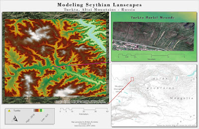
     This module is all about data preparation (for labs in the coming weeks) and starts our foray into landscape archaeology. We walked through gathering data for international landscapes from the USGS Earth Explorer. In particular, locating DEM data for an area in the Altai Mountains of Russia that contains known Scythian mound burials (also known as kurgans). For this exercise we used ASTER derived data. The Mosaic to New Raster tool was used to stitch together four raster datasets and from there we digitized a boundary and clipped the larger DEM down to something more manageable.
     The map deliverable shows the subset of data examined by way of a DEM symbolized with the elevation color ramp. It also highlights the area where the mounds are located with a georeferenced JPG.

This week's deliverable highlighting a region in the
Altai Mountains, Russia that contains burial mounds.

Special Topics: Module 4 - Predictive Modeling

     Predictive models are another tool in the archaeologists toolbox and this week we ran a simple predictive model for an archaeological district in Alaska. Predictive models can take many factors into account but for the purposes of this lab we used four components/generated surfaces: slope, aspect, elevation, and proximity to water. The Spatial Analyst extension is key in implementing a predictive model in ArcMap, particularly the Reclass, Surface, and Overlay toolsets (for the Weighted Overlay tool).
     While predictive models are great for informing survey decisions and streamlining cultural management processes they're aren't a panacea. They can in no way serve as substitute to boots on the ground, they can merely supplement and inform survey and project planning. There is no model, no matter how thorough, that can say that there are no archaeological materials in an area. These models represent probability and likelihood of the presence of archaeological remains.
     I am currently at the Great Basin Archaeological Conference and one of the presentations I was able to see discussed a predictive model for an area of National Forest that I work in. The model had a greater than 90% ability to predict the known site locations (it was thoroughly cross validated and I have spent the summer collecting data in some of the unsurveyed areas...it will be neat to see if the model predicted a comparable amount of density in that region). That being said, it's those sites that appear in the unlikely areas that become of great interest (in their deviation from a pattern).
     Yes, predictive models do not tell the whole story but they go a long way in helping, in my instance a National Forest, determine how best to allot limited resources (time, money, seasonal employees).
     Below is my map deliverable showing the areas that are likely to contain sites in green. That means their combination of slope, aspect, elevation, and proximity to water are ideal.

Map deliverable displaying the results of a predictive model
run using slope, aspect, elevation, and proximity to water.